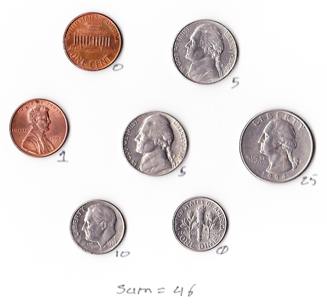
Imagine that you have a friend with 7 coins: some combination of pennies, nickels, dimes, or quarters. Your friend tells you that if you can guess the denomination of each of the coins, he will give them to you. He then proceeds to flip them onto the table, and to add the values of all the coins that land heads up, and tells you their sum. He agrees to repeat this process until you're confident in your answer.
#number of coins
physical_N = 7
#denominations of available coins, in cents
denominations = [1, 5, 10, 25]
#choose the value of the actual coins
physical_coins = np.random.choice(denominations, size = physical_N)
#probability that the coin will land heads (in this case, fair)
physical_pheads = np.ones(shape=physical_N)/2
#model of the physical system
Number_of_samples = 300
physical_measurement = np.array([np.sum(np.random.binomial(n=1,p=physical_pheads,
size=physical_N)*physical_coins)
for i in range(Number_of_samples)])
Now we can use our simulation to generate some test data:
samples: [12 41 11 45 22 27 36 17 41 21 ... ]
With seven coins, each able to take on four values, there are a total of 4^7 = 16384 different permutations. Luckily for us, symmetry dictates that not all of these solutions are unique: we don't care which coins are nickels and which are dimes, as long as we guess the correct number of each. In this case, we're interested in the combinations:
A large, but more manageable number. Each of these combinations represents a hypothesis (ie. two dimes, two nickels, two pennies, and a quarter) and together they form a 'hypothesis space'. For example, if we simplify the problem down to two coins, our probability space looks like a two dimensional matrix, with each coin represented along an axis, and the probability of the combination of those two coins making up the body of the table.

We translate the problem of guessing the coins to be a problem of filling in the question marks in this probability space with the probability that each particular combination represents the true value of the coins. As we have already seen, because we don't care about the order of the coins, our hypothesis space is redundant. In the picture above, the probability that the coins are worth 5 and 1 cent will be the same as the probability that the coins are worth 1 and 5 cents. To reduce the hypothesis space, we want to eliminate one of the symmetric hypotheses (5,1) and (1,5). One way we can do this is by saying that we will only look at coordinates that are in ascending order. This stipulation breaks the inherent symmetry of the problem and lets us look at the region of the hypothesis space with unique values. For the two dimensional case this makes our matrix:

We can generate this hypothesis space as a numpy array with seven dimensions (one for each coin) and each dimension of length four, one for each coin denomination.
potential_num_coins = physical_N
potential_coin_values = denominations
hypothesis_space_shape = [len(potential_coin_values)
for i in range(potential_num_coins)]
hypothesis_space = np.zeros(shape=hypothesis_space_shape)
it = np.nditer(hypothesis_space, flags=['multi_index'], op_flags=['readwrite'])
while not it.finished:
#are coordinates sorted?
if (sorted(list(it.multi_index)) == list(it.multi_index)):
it[0] = 1
it.iternext()
#normalize the state space
count = np.sum(hypothesis_space)
hypothesis_space /= count
We iterate over all elements of the array, setting all to zero except the ones whose coordinates come in ascending order. These we set such that their sum equals one, and they form a uniform prior hypothesis over the state space for us to apply Bayes rule and our data to.
In order to apply Bayes rule we need to define a likelihood function. The likelihood function gives us the probability of getting a certain value in each toss, given a specific hypothesis for the coins' individual values. To do this we can calculate all the different permutations of the coins falling heads up, looking for combinations that sum to the measured value. In python:
def likelihood(sum, coin_set_hypothesis):
p_heads = np.ones(len(coin_set_hypothesis))/2
p = 0
#the highest index we want is 2**len(bulbs)-1
for state in range(0,2**len(coin_set_hypothesis)):
#convert the state number to an array of individual coin states
st = np.array(map(int, bin(state)[2:].zfill(len(coin_set_hypothesis))))
value = np.sum(st*coin_set_hypothesis)
#accumulate the probabilities of permutations that result in the measured value
if value == sum:
p += np.product(st*p_heads + (1-st)*(1-p_heads))
return p
Now that we have data, a hypothesis space (with prior), and a likelihood function, we are ready to apply Bayes rule. For our problem, this takes the form:
So to apply the formula, when we get a new datapoint, we crawl over the entire hypothesis space, updating the probabilities of each hypothesis, and then we normalize the probabilities so that they sum to zero. In python, this becomes:
for datapoint in physical_measurement[:]:
it = np.nditer(hypothesis_space, flags=['multi_index'], op_flags=['readwrite'])
while not it.finished:
#only work on non-zero probabilities
if it[0]>0:
it[0] *= likelihood(datapoint, [potential_coin_values[i] for i in it.multi_index])
it.iternext()
#normalize
hypothesis_space /= np.sum(hypothesis_space)
# if we've reached a sufficiently high confidence, we can stop taking measurements
if np.max(hypothesis_space) > .999: break
measurement: 11 potential solutions: 72 prob of best guess: 0.0431965442765
measurement: 37 potential solutions: 30 prob of best guess: 0.0939334637965
measurement:  15 potential solutions:  18 prob of best guess:  0.212076583211
measurement:  31 potential solutions:  17 prob of best guess:  0.265437788018
measurement:  22 potential solutions:  12 prob of best guess:  0.246006006006
measurement:  26 potential solutions:  12 prob of best guess:  0.341038082771
measurement:  26 potential solutions:  12 prob of best guess:  0.400122469488
measurement:  36 potential solutions:  12 prob of best guess:  0.577365934659
measurement:  47 potential solutions:  9 prob of best guess:  0.64290385683
measurement:  40 potential solutions:  9 prob of best guess:  0.350104310773
measurement:  16 potential solutions:  9 prob of best guess:  0.379965178792
measurement:  21 potential solutions:  9 prob of best guess:  0.571889851959
measurement:  55 potential solutions:  4 prob of best guess:  0.518260091103
measurement:  35 potential solutions:  4 prob of best guess:  0.529247615951
measurement:  16 potential solutions:  4 prob of best guess:  0.521924746104
measurement:  21 potential solutions:  4 prob of best guess:  0.526892338442
measurement:  37 potential solutions:  4 prob of best guess:  0.539400203991
measurement:  30 potential solutions:  4 prob of best guess:  0.554541922563
measurement:  26 potential solutions:  4 prob of best guess:  0.510603887618
measurement:  55 potential solutions:  4 prob of best guess:  0.50891404123
measurement:  36 potential solutions:  4 prob of best guess:  0.578816353773
measurement:  36 potential solutions:  4 prob of best guess:  0.645292356054
measurement:  16 potential solutions:  4 prob of best guess:  0.580580572545
measurement:  47 potential solutions:  4 prob of best guess:  0.581762705335
measurement:  31 potential solutions:  4 prob of best guess:  0.513238821848
measurement:  47 potential solutions:  4 prob of best guess:  0.514291829821
measurement:  12 potential solutions:  4 prob of best guess:  0.514996238922
measurement:  16 potential solutions:  4 prob of best guess:  0.586513177343
measurement:  16 potential solutions:  4 prob of best guess:  0.654416532032
measurement:  46 potential solutions:  4 prob of best guess:  0.654606418732
measurement:  26 potential solutions:  4 prob of best guess:  0.587215897594
measurement:  42 potential solutions:  4 prob of best guess:  0.654720985541
measurement:  35 potential solutions:  4 prob of best guess:  0.587144733857
measurement:  26 potential solutions:  4 prob of best guess:  0.516254101845
measurement:  31 potential solutions:  4 prob of best guess:  0.615383141046
measurement:  30 potential solutions:  4 prob of best guess:  0.705670642705
measurement:  41 potential solutions:  4 prob of best guess:  0.761589968294
measurement:  46 potential solutions:  4 prob of best guess:  0.76176304029
measurement:  16 potential solutions:  4 prob of best guess:  0.810104284176
measurement:  16 potential solutions:  4 prob of best guess:  0.8505338556
measurement:  21 potential solutions:  4 prob of best guess:  0.85060579791
measurement:  15 potential solutions:  4 prob of best guess:  0.883616952898
measurement:  47 potential solutions:  4 prob of best guess:  0.883623423049
measurement:  40 potential solutions:  4 prob of best guess:  0.910098631886
measurement:  21 potential solutions:  4 prob of best guess:  0.910107783616
measurement:  30 potential solutions:  4 prob of best guess:  0.93821763582
measurement:  15 potential solutions:  4 prob of best guess:  0.952937925621
measurement:  25 potential solutions:  4 prob of best guess:  0.938221807153
measurement:  50 potential solutions:  4 prob of best guess:  0.910111271486
measurement:  16 potential solutions:  4 prob of best guess:  0.931033913426
measurement:  41 potential solutions:  4 prob of best guess:  0.947367831568
measurement:  20 potential solutions:  4 prob of best guess:  0.947368224558
measurement:  27 potential solutions:  4 prob of best guess:  0.93103434879
measurement:  21 potential solutions:  4 prob of best guess:  0.931034438103
measurement:  17 potential solutions:  4 prob of best guess:  0.947368397934
etc...
And now we can assess the value we arrived at using bayes law with the actual value from our model:estimated coin values: [1, 1, 5, 5, 10, 10, 25]actual coin values: [1, 1, 5, 5, 10, 10, 25]
estimated == actual? True