These entrepreneurs had realized early the advantage of A/B testing - trying multiple messages on a population to determine which would be more successful. Unfortunately I didn't have any cash with me, otherwise I would have stopped and
I would have liked to watch and see how these girls handled the balance between testing new messages vs. using the ones they had some confidence in. This is a pretty standard issue when testing and implementation phases of a project overlap: how to balance the exploration of options with exploitation of the leaders.
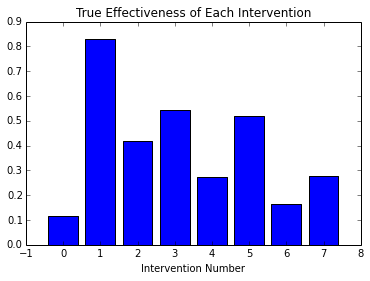
For instance, assume that I have a set of 'interventions', with the capacity to elicit a desired response - perhaps they are Facebook ads, and I want the viewer to respond by clicking the ad. Each intervention has an underlying effectiveness rate, which is the fraction of times the ad would be clicked out of all the times it was shown, if we were able to conduct an infinite number of experiments:
import numpy as np
num_trials = 30
results = np.random.binomial(n=1, p=true_effectiveness, size=(num_trials,num_interventions))
In this chart we see each intervention as a separate bar, with 30 trials conducted for each. Successful trials are in blue:
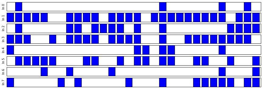
And we can also calculate a cost to conduct these tests (here counted as one per test) and the return we get having conducted them:

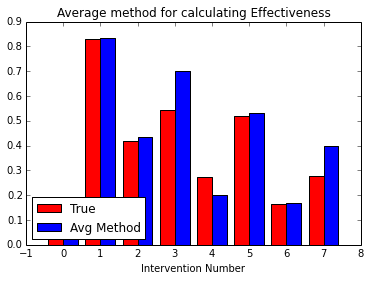
We see that having conducted about 240 trials, and received just over 100 positive responses, our average return is 42.5 percent.
Now, just averaging the values doesn't tell us very much about the uncertainty of our estimation - the true and estimated effectiveness in the chart above differ rather substantially. Modeling the response data as a Bernoulli random variable, with the effectiveness rate as its parameter, we can use Markov Chain Monte Carlo techniques to estimate what these distributions of effectiveness will look like:
import pymc as mc
bayes_effectiveness = mc.Uniform('bayes_effectiveness', lower=0, upper=1, size=num_interventions)
for i in range(num_interventions):
obs_i = mc.Bernoulli('obs_%s' % i, p=bayes_effectiveness[i], value=results[:,i], observed=True)
num_mc = 35000
mcmc = mc.MCMC( [bayes_effectiveness, obs_i] )
mcmc.sample( num_mc, 1000 )

Additionally, there is a significant amount of overlap, meaning that it is somewhat challenging to determine if one intervention is better than another. Based upon these distributions, however, we can calculate the probability that one intervention is better than another, by looking at the number of cases in the Monte-Carlo output in which that is the case:
A = np.array([mcmc.trace('bayes_effectiveness')[:,:]])
is_greater = np.sum(A > A.T, axis=1)*100./num_mc
This is a bit tricky to visualize. The chart shows the likelihood that the intervention represented by each column is more effective than the intervention represented by a particular row. Naturally the diagonals are zero, and blue, as an intervention can't be more effective than itself. The red squares - such as that at column 1, row 6 - show a high probability - in this case that intervention number 1 is highly likely to be superior to intervention 6.

But wait - that one out on the right, intervention 1, really does look better than most of the others, and the A/B chart we just drew shows that it's quite likely to be better than all of the rest. We don't really care about the true values of all of the distributions after all - what we care about is finding (with good confidence) the best of the set. What if we just took more trials of the ones that seem to be in the lead?
Well, it turns out there is a strategy like this in which as we get more information about the relative order, the more we rely on the leaders. It goes something like this:
1. For each intervention, choose a random value (0-1) based upon the distribution of its effectiveness
2. Choose the intervention with the highest random value, and conduct a trail using it
3. Update the intervention's distribution according to the result.
To simplify things, instead of computing arbitrary distributions, we'll specify that our results give a 'beta' distribution. This has the nice property that the probability can be computed analytically from two numbers: the total number of trials that have been performed for an intervention, and the number of successes that have resulted.
Implementing this algorithm in python is simple:
a = np.zeros([num_interventions,1]) # a is the number of successful trials of a particular intervention
b = np.zeros([num_interventions,1]) # b is the number of total trials of a particular intervention
for i in range(new_trials):
#randomly select an intervention proportional to its likelihood distribution
intervention = np.argmax(np.random.beta(1+a, 1+b-a))
#perform the experiment
result = np.random.binomial(n=1, p=true_effectiveness[intervention])
#update the priors
a[intervention] += result
b[intervention] += 1
We can then watch the results unfold over time. In the following animation, we see the distributions of each intervention develop over the same number of trials as we conducted above. As each intervention is tried, its distribution is highlighted. We can see that in the beginning, all distributions are relatively uniform, and so each intervention gets selected, randomly, with relatively high frequency.
As trials progress, we begin to get more resolution on which trials are better, and so these tend to be selected more regularly, and our estimate of their underlying true effectiveness improves. The distributions for the best results get tighter. We still try the other interventions from time to time, proportional to how likely they may be to overthrow the reigning champion. This makes the algorithm more robust to the random chance that a winning distribution got off to a bad start, and in the case of an intervention whose behavior changes over time, gives us a chance to correct ourselves.
Now, just for fun, lets see what happens if we add a new intervention to the mix. Intervention 8 arrives after 240 trials have already been conducted, and probability distributions have been developed for interventions 0-7. In the course of continued testing, 8's distribution jumps around a lot more than those of 0-7, as it works to get established.

For more info on PyMC and this particular problem, check out Bayesian Methods for Hackers.