When I first learned about Bayes Law, it was through algebraically manipulating the symbols in the equation until I'd convinced myself that the equation was algebraically correct.
This is totally different from forming an intuition about why Bayes Law should hold. Here's a more visual/spatial representation, which might be more helpful.

First, consider a space that contains all of the events that could possibly occur in the universe. We'll represent that space in two dimensions, and draw a line around it, and call that space 'U':
In this universe, we'll have an event (say, that I eat an apple today) and we'll call it 'A'. This event takes up some finite space in the universe of all possible events, here shown in red:
The amount of area that the event A takes up in the space U is the probability of the event occurring. Think of it this way - suppose I pick a random point somewhere in the space U. If that point is within the red region, then event A occurs, and if it falls outside of the red region, event A does not occur.
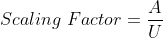
Clearly as the size of the red area increases, there is a higher likelihood that 'A' will occur. This probability can be expressed as a ratio of the areas of A to U:
Now lets suppose another event (say, that I eat a banana today) we call 'B'. The event B is partially overlapping with event A, and so our universe now has four possible outcomes: A occurs alone, B occurs alone, both A and B occur together, or neither A or B occur.
We can express the joint probability of A and B occurring as the ratio of the area of the AB region to the universe U, and what we discussed about choosing random points in or outside of this region holds:
Now lets say we don't actually know how much of the area of U (the universe) that the region AB takes up, but we do know the amount of area A (the red region) that AB takes up. We can think about this as having 'zoomed-in' on the red region:
The space within the red region that the AB region takes up is known as the conditional probability of AB given A:
If we want to recover the unconditional probability, then we just need to 'zoom out' again to look at the full universe U. To do this, we scale the conditional probability down by the ratio of the red area to the total area:
so that we have:
Now bayes law takes this scaling idea one step further, and asks what the probability of AB is given B. We can repeat our last operation in reverse, zooming in on the blue region:
When we do this zoom in, we can find the conditional probability of AB given B, and write it in terms of the independent probability of AB. The scaling factor to zoom in to B is of course the inverse of the factor to zoom out:
Now we can combine the two steps, beginning with the conditional probability of AB given A, zooming out to the full universe U, and then zooming back in to just area B to find the probability of AB conditioned on B:
And substituting in our probability notation:
Which is what we'd hoped to find, Bayes Law:
To summarize - in operating Bayes Law, we take the probability that an event will occur when we restrict our attention to the conditional event. We then scale that probability to the independent probability of that event occurring in the entire universe by zooming out from our initial restricted region. Then we zoom in again on a different region, to find a different conditional probability.