James Houghton - Brian Arthur's Lock-in
With a few modifications, the discrete time, agent model presented in Arthur, W. Brian. “Competing technologies, increasing returns, and lock-in by historical events.” The economic journal 99.394 (1989): 116-131. can be represented using stock and flow notation that lets us understand the feedback loops present.
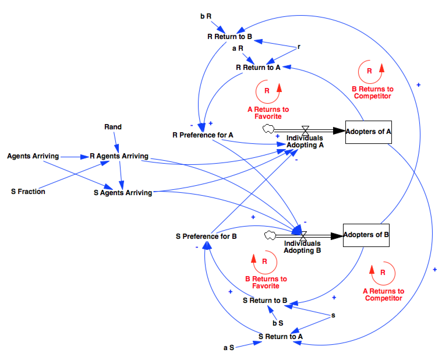 The general feedback structure of the model consists of a number of reinforcing (given positive parameters) feedback loops for two categories of actor, serving to drive their adoption patterns to the technology with a larger installed base.
The feedback gains are controlled by parameters r and s which Arthur uses to specify three regimes for the model - increasing returns to adoption, constant returns to adoption, or diminishing returns to adoption - each of which has its own unique behavior.
%pylab inline
import pysd
import pandas as pd
import numpy as np
model = pysd.read_vensim('Arthur - 1989 - Competing Technologies.mdl')
def rand():
    return np.random.rand()
model.components.rand = rand
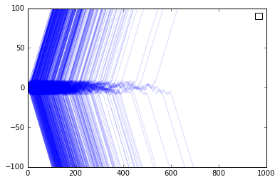
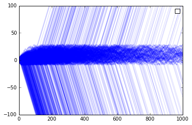
Increasing Returns to Adoption
With r and s positive, and actors R and S having different preferences for the goods, when one technology or the other reaches a certain threshold, it attracts both kinds of customers R and S, due entirely to volume. The likelihood that a trajectory will cross this threshold at time t is defined by the properties of the random walk effective between the thresholds.
A = []
B = []
n_sim = 1000
for i in range(n_sim):
    res = model.run(params={'r':.1,
                            's':.1,
                            'b_r':1,
                            'b_s':2,
                            'a_r':2,
                            'a_s':1},
           return_timestamps=range(1000))
    A.append(res['adopters_of_a'])
    B.append(res['adopters_of_b'])

Adf = pd.DataFrame(A).T
Adf.columns = range(n_sim)
Bdf = pd.DataFrame(B).T
Bdf.columns = range(n_sim)

(Adf-Bdf).plot(color='b', alpha=.15)
plt.legend([])
plt.ylim(-100,100)
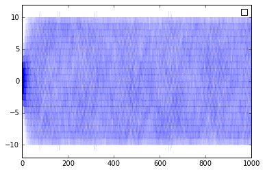
Decreasing returns to adoption
When both products show decreasing returns to scale, Arthur’s paper demonstrates that the thresholds become stabilizing, as opposed to destabilizing, as at each point both types of consumers choose to use the less popular product. This might be the case for goods in which exclusivity confers status on the good. This could be the case for products competing in the micro-brew market, where the ‘cachet’ associated with particular goods decreases as it becomes more widely consumed. (Thus, hipsters as a stabilizing influence on the economy.)
A = []
B = []
n_sim = 1000
for i in range(n_sim):
    res = model.run(params={'r':-.1,
                            's':-.1,
                            'b_r':1,
                            'b_s':2,
                            'a_r':2,
                            'a_s':1},
           return_timestamps=range(1000))
    A.append(res['adopters_of_a'])
    B.append(res['adopters_of_b'])

Adf = pd.DataFrame(A).T
Adf.columns = range(n_sim)
Bdf = pd.DataFrame(B).T
Bdf.columns = range(n_sim)
(Adf-Bdf).plot(color='b', alpha=.005)
plt.legend([])
plt.ylim(-12,12)
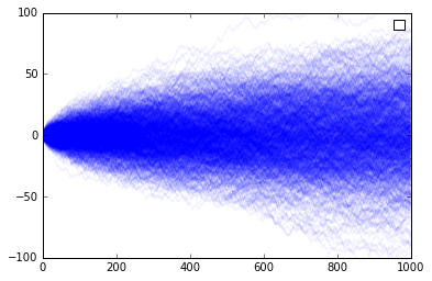
Constant returns to Scale
When there is no influence between the current adoption and future adoption - i.e. no returns to scale whatsoever - then the trajectory is that of a random path as would normally be found between the bounds of the model.
A = []
B = []
n_sim = 1000
for i in range(n_sim):
    res = model.run(params={'r':0,
                            's':0,
                            'b_r':1,
                            'b_s':2,
                            'a_r':2,
                            'a_s':1},
           return_timestamps=range(1000))
    A.append(res['adopters_of_a'])
    B.append(res['adopters_of_b'])

Adf = pd.DataFrame(A).T
Adf.columns = range(n_sim)
Bdf = pd.DataFrame(B).T
Bdf.columns = range(n_sim)
(Adf-Bdf).plot(color='b', alpha=.05)
plt.legend([])
plt.ylim(-100,100)
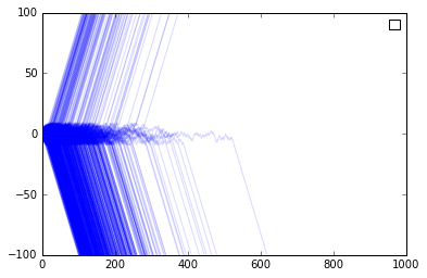
When there is net preference
The article talks about times in which an objectively better technology would come to dominate. This is actually difficult to operationalize in Arthur’s model, as if both types of agents agreed that a product was better, then it will always dominate. We can try to demonstrate with a ‘net preference’, in which one group has a larger preference for one product than the other group has for the product’s competitor.
Here we give one party twice the overall preference of the other for its favored good. This shows unsurprisingly that in the majority of cases, the product of stronger preference wins - but not always. We see this manifest as a lower threshold beyond which the lock-in takes place.
A = []
B = []
n_sim = 1000
for i in range(n_sim):
    res = model.run(params={'r':.1,
                            's':.1,
                            'b_r':1,
                            'b_s':4,
                            'a_r':2,
                            'a_s':1},
           return_timestamps=range(1000))
    A.append(res['adopters_of_a'])
    B.append(res['adopters_of_b'])

Adf = pd.DataFrame(A).T
Adf.columns = range(n_sim)
Bdf = pd.DataFrame(B).T
Bdf.columns = range(n_sim)
(Adf-Bdf).plot(color='b', alpha=.15)
plt.legend([])
plt.ylim(-100,100);
Another way to investigate this would be to give one group a larger population, such that a larger fraction of all people prefer a particular technology. Here we make the number of S consumers slightly larger than that of the R consumers. We see again that the more popular side is favored, but cases are not rare where the less popular technology wins the market.
A = []
B = []
n_sim = 1000
for i in range(n_sim):
    res = model.run(params={'r':.1,
                            's':.1,
                            'b_r':1,
                            'b_s':2,
                            'a_r':2,
                            'a_s':1,
                            's_fraction':.55},
           return_timestamps=range(1000))
    A.append(res['adopters_of_a'])
    B.append(res['adopters_of_b'])

Adf = pd.DataFrame(A).T
Adf.columns = range(n_sim)
Bdf = pd.DataFrame(B).T
Bdf.columns = range(n_sim)
(Adf-Bdf).plot(color='b', alpha=.15)
plt.legend([])
plt.ylim(-100,100);
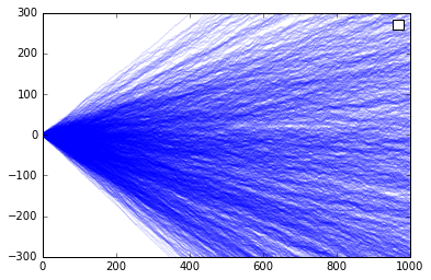
Relaxing some assumptions
As the model is currently constructed, the individuals in each category have the same level of preference for the good, and so for increasing returns, the zone between the lock-in thresholds is characterized by pure random walk, as individuals arrive.
It is more likely that individuals will have varying degrees of concern for the current level of adoption. If we replace the r and s parameters, each timestep, with a value drawn from an exponential distribution with the same average value as our previous simulations, we get some rather unusual results.
The threshold itself seems to disappear, as there will always be someone who is willing to buck the trend - they are just more and more rare. Instead of a threshold beyond which behavior shifts for all users, we see a more continuous progression without a true point of no return, merely a general trend.
def rand():
    return np.random.exponential(scale=.1)

model.components.r = rand
model.components.s = rand
A = []
B = []
n_sim = 1000
for i in range(n_sim):
    res = model.run(params={'b_r':1,
                            'b_s':2,
                            'a_r':2,
                            'a_s':1},
           return_timestamps=range(1000))
    A.append(res['adopters_of_a'])
    B.append(res['adopters_of_b'])

Adf = pd.DataFrame(A).T
Adf.columns = range(n_sim)
Bdf = pd.DataFrame(B).T
Bdf.columns = range(n_sim)
(Adf-Bdf).plot(color='b', alpha=.15)
plt.legend([])
plt.ylim(-300,300);
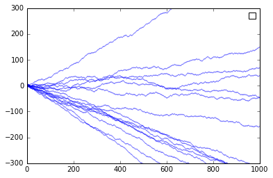
The individual traces essentially say that we lock into the ratio that is established early on, not necessarily to one product or the other.
(Adf-Bdf)[range(15)].plot(color='b', alpha=.5)
plt.legend([])
plt.ylim(-300,300);
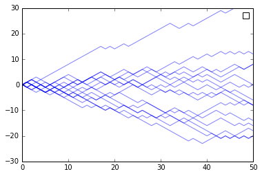
Looking at the start of the timeseries, we see that similar chances suggest the final outcome.
(Adf-Bdf)[range(15,30)].plot(color='b', alpha=.5)
plt.legend([])
plt.ylim(-30,30);
plt.xlim(0,50)
Why are we even doing this?
If we were able to make a well calibrated prediction of the likelihood that one technology would win over the other (e.g. on day 20, give 65% likelihood of technology A) then we could set betting lines for investment. What we want to do is to infer distributions for the model parameters based upon the time history so far. If the process is truly a random walk, then we don’t get any information out of it (other than if there is an imbalance in populations R and S). If however, we allow for individual variation, we break the symmetry of the random walk and may be able to infer something about the model parameters (or at least the hyper-parameters of the random distributions). Thats for another day.